Our mission is to become the Number 1 CRO in the country providing supplementary services for clinical trials and ultimately help our clients to make affordable and quality health care to the masses a reality.
21.6.21
Our mission is to become the Number 1 CRO in the country providing supplementary services for clinical trials and ultimately help our clients to make affordable and quality health care to the masses a reality.
1.7.10
Dynamic concatenation of transposed variables
Prepared by Jose Abraham
The transpose procedure in SAS changes multiple values in rows (for a column) into columns, and can also change multiple columns’ values into multiple rows values for a single column. The number of variables (columns) to be created in the output file is based on the maximum number of observations (rows) in a variable (column) to be transposed. If the prefix= option is not specified, then the transposed variables have names Col1, Col2 etc…. i.e. if the dataset has 4 observations in a variable, then on transposing 4 variables namely Col1, Col2, Col3 and Col4 are obtained against each value of the by variable (labparam, lab_id in the below example).
In certain situations, it is required to concatenate the columns obtained during transposing. This can be attained simply by setting the dataset and concatenating the variables using the concatenation operator (||).
e.g. Newvar= Col1|| ‘,’||Col2|| ‘,’||Col3|| ‘,’||Col4;
This procedure may however not produce desirable results if any of the four columns have missing values. If suppose Col3 and Col4 have missing values then consecutive ‘,’ will be presented as the last few characters in the variable Newvar.
The concatenation is thus done by determining the maximum number of Col variables in the transposed dataset and then concatenating the non missing variables to create the new variable against each of the by variables.
Consider the following example from a clinical trial analysis, where the laboratory values are collected at different laboratories. For different laboratories, the reference ranges adopted for parameters are different.Such a dataset is shown below
While obtaining descriptive statistics for different lab parameters, the lab ranges are to be presented in the report as a sub header of the following form.
e.g. Param1
Lab-A: 0-35 g/L (Age 0-99)
Lab-B: 0-34 g/L (Age 0-18), 0-35 g/L (Age 18-60), 0-36 g/L (Age 60-99)
For different laboratory groups the number of ranges will be different, so it is necessary to dynamically concatenate the ranges for each lab for each parameter. The steps involved in this process are given below
Dataset with the lab ranges is transposed.
*Transposing the data to get the reference ranges horizontally;
proc transpose data=range out=range_trn;
by labparam lab_id;
var range;
run;
Select the information about the number of columns in the transposed dataset with the help of sashelp.vcolumn dataset. A macro variable named ‘coln’ is created with the maximum number of ‘Col’ variables as its value.
*Creating a macro variable with maximum number of columns;
data _null_;
set sashelp.vcolumn end=last;
where trim(libname) = 'WORK' and trim(memname) ='RANGE_TRN' and upcase(substr(name,1,3))='COL';
if last then call symput('coln',trim(left(put(_n_,6.))));
run;
Set the transposed dataset and giving array reference to the ‘Col’ variables. Concatenate the ranges with using a do loop and then remove the preceding comma by taking substring of the concatenated variable. A variable named ‘labrange’ is created by concatenating with the lab_id.
data range_con;
length convar $400;
array cols {&coln.} $50 col1-col&coln.;
set range_trn;
do i=1 to dim(cols);
if not missing(cols[i]) then convar= trim(convar)||', '||cols[i];
end;
convar=substr(left(convar),2);
Labrange=trim(left(lab_id))||':'|| compbl(convar);
keep labparam lab_id labrange;
run;
The dataset range_con contains the concatenated ‘labrange’ variable.
*Transposing the dataset to present the ranges for different lab_id's in different variables;
proc transpose data= range_con out=lab_rng(drop=_name_);
id lab_id;
by labparam;
var labrange;
run;
The output dataset obtained during transposing is of the following form
By merging it with the descriptive statistics dataset and using ‘labparam’ and the variables containing the concatenated lab ranges (here LAB_A and LAB_B) as by variables in proc report creates a report which contains descriptive statistics for one parameter per page. By using the ‘#byval’ option in the title statement we can obtain the sub headers of the following type.
Param1
Lab-A: 0-35 g/L (Age 0-99)
Lab-B: 0-34 g/L (Age 0-18), 0-35 g/L (Age 18-60), 0-36 g/L (Age 60-99)
Project specific SAS shortcuts
Prepared by Jose Abraham
As a SAS programmer, an important concept to know when opening and saving SAS programs is the ‘SasInitialFolder’. The location of this folder is the path name where SAS reads or stores files when a specific drive and pathname is not given. The name of this path appears in a small panel located in the lower right-hand corner of our SAS session. This can be changed at any time with a double-click within that rectangle to access a dialogue box, then entering the drive and path to the desired folder in the space provided or by moving through the folders as done while searching for a particular file. But the change which is made is not permanent. During the next invocation of the SAS System, the current folder will by default present the current folder path that was permanently set. In SAS v8 for windows, the default folder may be something like “C:\Documents and Settings\<user name>\My Documents\My SAS Files\V8” or a path which is in the drive where SAS is installed (e.g. “E:\SAS Installation”). When trying to open or save a program in a SAS session, this default folder will be shown and changing this folder to the desired folder may consume some amount of our valuable time. Here is the way to save this time and also to make project specific SAS shortcuts, which will allow opening and saving SAS programs of that project from the ‘SAS Programs’ folder which is set for that project. The steps to set the current folder to a new location are given below. The folder which is to be set should be created before going through the following steps. 1. Create a shortcut of SAS by clicking on the ‘Start’ menu and select ‘SAS’ from ‘All Programs’, right click on it and then select ‘Send to Desktop’. Then a new SAS shortcut icon will be created in the desktop.2. Right click on the icon and select ‘Rename’ and give a name related to the project.3. Again right click on the icon and select ‘Properties’ and click on the ‘Shortcuts’ tab.4. In the ‘Target’ box, go to the far end of the right-hand side of what is seen in that by pressing the ‘End’ button. Type one space, and enter the following command exactly as you see it here: -sasInitialFolder="."5. The current or working SAS folder will be the pathname that is specified in the 'Start in' field (located just below the 'Target' field). To designate the choice of the current folder, enter the drive and pathname of it within that box. This folder needs to exist on the specified directory.e.g. “G:\Project1\SAS programs”6. Click on ‘Apply’ and then click ‘OK’. The shortcut is now ready for use for the particular project and it will direct to the specified folder on clicking ‘File-> Open’ or ‘File->Save As”.
8.6.10
Index, Indexc and Indexw functions
Prepared by Meena R S
The INDEX, INDEXC and INDEXW functions are used for determining the character matches. These functions are useful for testing purposes. The index and indexc functions can indicate if a string of characters is present in a target variable. Both functions return the position number of the match in the target variable. A zero indicates that the search argument is not present in the target variable.
For finding a special character such as a letter, a group of letters, or special characters, Index functions can be used and it is case sensitive. The syntax is,
INDEX (source, excerpt)
The INDEXC function allows multiple arguments and will identify the first occurrence of any of the characters in any of the arguments, but otherwise functions similarly to the index function.
/* Example: 1 */
/* Results*/
The INDEXW function searches source, from left to right, for the first occurrence of excerpt and returns the position in source of the substring's first character. If the substring is not found in source, INDEXW returns a value of 0. If there are multiple occurrences of the string, INDEXW returns only the position of the first occurrence.
The INDEXW function is case sensitive function that performs exactly the same function as the INDEX function, with one significant exception. The indexw function searches for strings that are words, whereas the index function searches for patterns as separate words or as parts of other words.
/* Example: 2 */
/* Results */
Result Explanation
The above program demonstrates the difference between INDEX and INDEXW functions. In the first observation in the table above, the INDEX function returns a 1 because the letters "the" as part of the word "there" begin the string. Since the INDEXW function needs either white space at the beginning or end of a string to delimit a word, it returns a 12, the position of the word "the" in the string. Observation 3 emphasizes the fact that a punctuation mark does not serve as a word separator. Finally, since the string "the" does not appear anywhere in the fourth observation, both functions return a 0.
Read from multiple external files in one data step by using FILEVAR= option
Prepared by Jose Abraham
External files are usually read into SAS one by one using separate data steps for each external file. But multiple external files which have the same structure can be easily read into SAS in one data step by using FILEVAR= and END= options in the INFILE statement. Following example illustrates how to read multiple external files where the locations of the external files are stored in another external file.
Consider we have demographic information of subjects from three different centers stored in three external files. All the three external files have the same structure as given below


The data values are aligned in columns and there are no missing values. The layout follows.
We have another external file which contains the location information of these external files. Suppose these files are stored in the 'demog' folder in the E-drive, and the following external file (dmgfiles) which contains the locations is also in it.
Following SAS data step reads the three external files in one DATA step by using the names which are specified in the external file 'dmgfiles'. This reads the list to determine the external files it should read.
Data step working:
1.First INFILE statement specifies the name of the external file containing the list of filenames that the DATA step should read.
2.First INPUT statement reads the name of the external files with modified list input. A width (60) which is sufficient to hold the name of the external file is specified.
3.Second INFILE statement specifies a text, dummy, and this act as a placeholder for the file specification which is always required on the INFILE statement. The actual specification for the input file comes from the value of the variable assigned by the FILEVAR= option.
a.The FILEVAR= option is set to 'dmgfiles', the variable that contains the name of the external file that the current iteration of the data step should read.
b.END= option defines a variable that SAS sets to 1 when it reads the last data line in the currently opened external file. The END= variable is initialized to 0 and retains the value until it detects that the current input data line is the last in the external file. SAS then sets the variable to 1.
c.When the FILEVAR= option is included in the INFILE statement, SAS resets the END= variable to 0 when the value of the FILEVAR= variable changes (If SAS did not reset the value of the END= variable to 0 each time it opened a new external file, the DATA step would stop after reading the first external file).
4.The do while loop is controlled by testing the value of the END= variable. The loop stops after SAS reads the last data line in the currently opened external file.
5.Name of the file from which the records are read (source file name) is assigned into a variable 'Source'.
6.The above data step iterates four times: one for each of the dmg files (dmg01, dmg02, dmg03) and a fourth time in which it detects that there are no more data lines in the external file that contains the filenames.
7.The default behavior of SAS is that it writes an observation to a data set only at the end of each iteration of the DATA step. An explicit OUTPUT statement is specified to avoid this and output all data values read form the external file.
8.The output dataset 'demogdat' obtained is as follows
Ctrn | Subjid | Age | Sex | Race | |
E:\demog\dmg01.txt | 001 | 001_01 | 29 | Male | Caucasian |
E:\demog\dmg01.txt | 001 | 001_02 | 28 | Female | Caucasian |
E:\demog\dmg01.txt | 001 | 001_03 | 25 | Male | Caucasian |
E:\demog\dmg02.txt | 002 | 002_01 | 27 | Male | Asian |
E:\demog\dmg02.txt | 002 | 002_02 | 28 | Male | Asian |
E:\demog\dmg02.txt | 002 | 002_03 | 25 | Female | Asian |
E:\demog\dmg03.txt | 003 | 003_01 | 27 | Female | Asian |
E:\demog\dmg03.txt | 003 | 003_02 | 28 | Male | Asian |
E:\demog\dmg03.txt | 003 | 003_03 | 25 | Female | Asian |
21.8.09
Macro Variable Resolution Using Multiple Ampersands
Prepared by Meena R S (meena@kreara.com)
The SAS macro consists of two basic parts: macros and macro variables. The names of macro variables are prefixed with an ampersand (&) while the names of macros are prefixed with percent sign (%). Prior to the execution of the SAS code the macro variables are resolved. The resolved values are then substituted back into the code.
The macro variable references that have been described with one ampersand preceding the macro variable name are direct reference to a macro variable. In indirect referencing, more than one ampersand precedes a macro variable reference. The macro processor follows specific rules in resolving references with multiple ampersands.
The rules that the macro processor uses to resolve macro variable reference that contain multiple ampersands follow
- Macro variable references are resolved from left to right
- Two ampersands (&&) resolve to one ampersand (&)
- Multiple leading ampersands cause the macro processor to rescan the reference until no more ampersands can be resolved.
Consider the example below.
Options symbolgen;
%let section4 =operating system;
%let n=4;
%put &§ion&n;
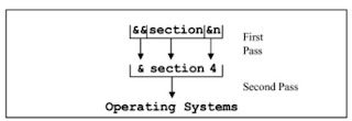
For the above code, on the first pass the two ampersands are resolved to one and &n is resolved to 4, yielding §ion4. On the second pass the macro variable reference §ion4 resolves to operating system.
The following figure shows the process of resolving the macro variable reference in the program.

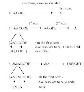
%let a =freight;
%let b=passenger;
%let c=special;
%let code=a;
%put &code;
%put &&code;
%put &&&code;
The following demonstrates how the macro variables with multiple ampersands are resolved.

Combining SAS data sets using UPDATE statement
UPDATE is an executable type SAS statement generally used in DATA steps. By updating a SAS dataset replaces the values of variables in one dataset with values from another dataset. The dataset containing the original information is the master data set, and the data set containing the new information is the transaction data set. UPDATE performs much the same function as merge with two exceptions:
Ø Only two datasets can be combined using UPDATE statement
Ø If the observation of a variable in the transaction dataset (i.e. data set containing new information) is missing, then the updated dataset containing the value of the observation same as in the master dataset
Syntax
DATA updated data set;
UPDATE master-data-set transaction-data-set;
BY variable-list;
RUN;
Where Master-data-set names the SAS data set that is used as the master file. Transaction-data-set names the SAS dataset that contains the changes to be applied to the master data set. Variable-list specifies the variables by which observations are matched.
Basic use of UPDATE statement
Consider two datasets, Lab1 and Lab2. Both data sets have four subjects with information about their blood pressure at two different times. The first dataset Lab1 contains the subject id, name of the subject and Blood pressure reading. The second dataset contain the latest blood pressure reading for the same subjects but the name of the subjects is not given.
It is required to replace the latest Blood pressure values in LAB1 with the values in LAB2. Here LAB1 is known as Master data set and LAB2 is transaction dataset.
Subject Name BP
001 AAA 120
002 BBB 130
003 CCC 140
004 DDD 150
Lab 2
Subject BP
001 160
002 160
003 160
004 160
The following program updates LAB1 (Master Dataset) with LAB2 (Transaction dataset).
DATA lab1_updated;
UPDATE lab1 lab2;
BY Subject;
RUN;
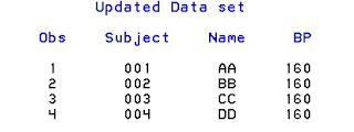
Printed output of lab1_updated is given below;

In the above example it is found that the latest blood pressure value is populated into updated dataset based on the BY variable Subject identifier.
Suppose Lab1 contains a duplicate observation. For example,
Lab 1
Subject Name BP
001 AAA 120
002 BBB 130
002 BBB 130
003 CCC 140
004 DDD 150
DATA lab1_updated;
UPDATE lab1 lab2;
BY Subject;
RUN;
If the above program is executed updating will not work for duplicate BY value.
That means if master data set contains two observations with the same value of the BY variable, the first observation is updated and the second observation is ignored. SAS writes a warning message to the log when the data step executes.
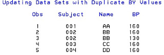
Printed output of lab1_updated is given below;

Observations two and three have duplicate values of BY variable subject identifier. However, the value of variable Blood pressure was not updated in the second occurrence of the duplicate BY value.
A situation may arise where a missing observation can occur in master dataset or in transaction dataset. Below example illustrates updating when dataset contains unmatched and missing observations.
Lab A
Subject Name BP
001 AAA .
002 BBB 130
003 CCC 140
004 DDD 150
Lab B
Subject BP
001 160
002 .
003 160
004 160
In the above dataset Lab A (Master Dataset) contains missing value corresponding to the subject 001 and the Lab B (Transaction dataset) contains missing value corresponding to the subject 002. The output of the below code gives the latest known BP value for each subject.
DATA lab1_updated;
UPDATE LabA LabB;
BY Subject;
RUN;
Printed output is given below;

The following is a more advanced example where the UPDATE statement is used to “flatten” a dataset containing different variable data values for a key spread across several observations. The goal is to combine non-missing values into one record per unique key value. The master dataset structure is read, but the OBS=0 option stops the DATA step from reading any data from it. The same dataset is then uploaded as transaction dataset, flattening non-missing observations for each unique key into one observation.
DATA lab;
INPUT Subject $ Calcium Albumin Chloride;
CARDS;
001 2.25 . .
001 . 49 .
001 . . 100
002 3.1 . .
002 . 50 90
002 . . .
;
RUN;
DATA lab;
UPDATE lab (obs=0) lab;
BY subject;
RUN;
Output is given below;

